The Bias-Variance Tradeoff
The Bias-Variance Tradeoff is one of the most fundamental concepts in Machine Learning. Understanding this tradeoff is the key to develop an intuitive sense of how to tune your models whose job is to accurately model the underlying data distribution.
But what exactly is this tradeoff? When we train our model we measure how well it performs on the data that we use to train it on. This error is called training error.
However, what we really care about is test error, the error when predicting the response variable for new data that our model hasn't seen before!
When trying to optimize for training error we will eventually start to overfit to noise in the underlying data distribution we are trying to model. So while our training error is close or at zero it might do terribly on the test data! The hard part is finding the sweet spot where our test error is minimized. It is important to remember that you can never train on the test data!
We can characterize this tradeoff as follows:
1. How much can we minimize training error
2. How well does the training error approximate the test error
But how exactly do bias and variance relate to this tradeoff?
They are the two source of errors in our test error and it is impossible to optimize for both.
Bias: The error due to bias is taken as the difference between the expected (or average) prediction of our model and the correct value which we are trying to predict.
Variance: The error due to variance is taken as the variability of a model prediction for a given data point.
-- Scott Fortmann-Roe [link]
So we can think of the bias as the expected difference between our average model prediction and the true data distribution. Is our model complex enough to capture the intrincities of the underlying data distribution? If our bias is high our model is said to underfit we are using too simple of a model.
The variance however is characterized by how consistent our model is. If we would build our model for a large number of training sets would it consistently do good or would its results vary? If our model is too complex for the underlying data distribution we start to overfit.
It is intuitive to think about the tradeoff as a dartboard. Each dart you throw is your model trained on a new set of training data. The closer the darts are to the center the more accurately they are modelling the underlying data distribution. Also, as they get more dispersed it means that your model is overfitting to noise and is not consistent in its accuracy.
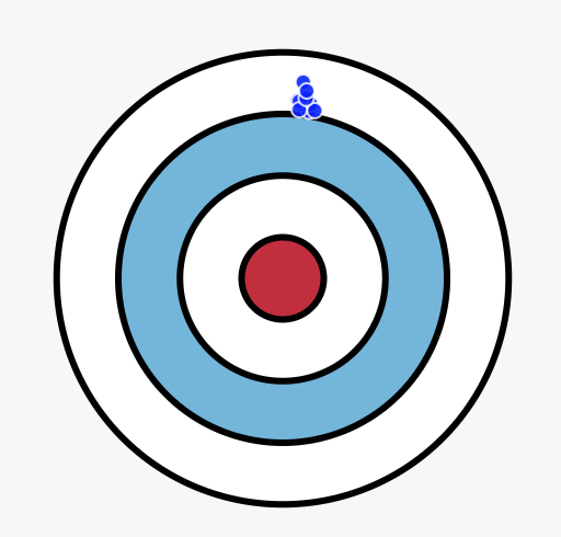
High bias but low variance
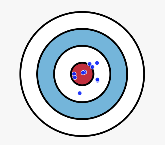
Low bias but high variance
K-nearest neighbours
To explain the bias-variance tradeoff our playground above employs the K-nearest neighbour classification algorithm. The algorithm takes a training dataset consisting of labeled points in Euclidean space that belong to one of two classes, the blue class or the orange class. The algorithm classifies new data by checking the majority class of the k nearest points. The choice of k> is highly related to the bias variance tradeoff. How do you think the choice of k affects it?
You can adjust how much noise there is in the dataset, more noise will make it harder for your model to model the true signal in the data. The training and test error is displayed for each of your choice of k as well as the decision boundary, telling you exactly how new points would be classified On the right there is the aforementioned dartboard for assessing the bias and the variance. For each noise and k parameter we run the model on numerous training sets generated from the same underlying distribution. We then visualize each model as a dart, remember it is not only best to hit close to the center but also to show consistency.
Go ahead and play with k-nearest neighbours at the playground at the top of this page before we reveal to you the true distribution we used to model the data for the playground.
Uncovering the true distribution
So by now you hopefully have some idea about how the choice of k affects the bias-variance tradeoff. Before we dive into the choice of k however, let's talk about the data that you played around with using the playground.
The data is carefully simulated, in fact it's simulated to (usually) make a non-linear decision boundary between the two classes. The data simulation technique is the one used in Elements of Statistical Learning [link], a book I highly recommend, to show how K-nearest neighbours outperforms linear models.
First we establish two Gaussian distributions for each class. One with a mean of (0.5,-0.5) and the other one with a mean of (-0.5,0.5), both having identical constant covariance matrices. We then sample 10 points from each distribution. These 20 points become the means of new distributions, that is 10 distributions for each class. All of those distributions have an identical covariance matrix that scales proportionately with the noise parameter in the playground. It is good to think of them as cluster centroids. Then, for 200 points for each class we pick one of the 10 distributions for the respective class at random and sample a point from it. This becomes the training dataset. For the test dataset we do exactly the same thing.
The data generation process can be visualized below. The big circles are the meta-distributions for each class. The points sampled from them become the cluster means for each class. And finally we can see the data being sampled
Now that the underlying mechanics operating the mysterious data distribution have been unveiled. What is the optimal choice of k? And how do we find it?